Identifying Major Players in Endangered Wildlife Trade
Problem Description
Since the Stone Age, mankind has turned to nature for food, commerce and companionship. Our impact back then was minimal as resources were consumed at sustainable rates. However, over the past few decades, nature is increasingly under threat from overconsumption and excess capitalism. Our planet is facing multiple challenges on the environmental front, ranging from global warming to forest degradation.
One corrosive impact of our greed is the shrinking wildlife diversity and population. In 2000, IUCN counted a total of around 10,000 endangered species. By 2017, this number has doubled to 24,431 species. In the face of such overwhelming statistics, it is imperative for us to take action and protect these species from extinction. In this project, we will aim to contribute by using data from both CITES (Convention on Internation Trade in Endangered Species of Wild Fauna and Flora) and IUCN to identify the major players behind endangered wildlife trade.
To skip the methodology and proceed straight to the results, please click here.
Preliminaries
First load the necessary packages for this exercise.
# Disable scientific notation
options(scipen=999)
# Load default settings for R Markdown -- see file for more details
source("shared/defaults.R")
# Load some helper functions
source("shared/helper.R")

options(stringsAsFactors = FALSE)
# To install streamgraph, use devtools::install_github("hrbrmstr/streamgraph")
# To install rgdal, you may need to follow these instructions on Mac
# https://stackoverflow.com/questions/34333624/trouble-installing-rgdal
# (Kudos to @Stophface)
packages <- c("dplyr","ggplot2","tidyr","pander","scales","DiagrammeR","data.table","parallel",
              "htmlwidgets","streamgraph","purrr","EnvStats", "waffle","sunburstR",
              "leaflet","colorspace","toOrdinal","igraph","ggraph","grDevices","sf")
load_or_install.packages(packages)

data_dir <- "data/"
specs_dir <- "specs/"

si <- sessionInfo()
base_pkg_str <- paste0("Base Packages: ",paste(si[["basePkgs"]], collapse=", "))
attached_pkg_str <- paste0("Attached Packages: ",paste(names(si[["otherPkgs"]]), collapse=", "))
cat(paste0(base_pkg_str,"\n",attached_pkg_str))
## Base Packages: parallel, stats, graphics, grDevices, utils, datasets, methods, base
## Attached Packages: sf, ggraph, igraph, toOrdinal, colorspace, leaflet, sunburstR, waffle, EnvStats, purrr, streamgraph, htmlwidgets, data.table, DiagrammeR, scales, tidyr, pander, ggplot2, rlang, dplyr, knitrAbout the Data
We will be using wildlife trade data from CITES for the period of 2001 to 2015, with the following caveats:
- 2016 and 2017 were excluded due to data lag in the year of analysis (2018). (See Section 1.2.2 of the guide for more details.)
- Analysis will be restricted to trades whose sources originated from the wild.
Listed below is an overview of the CITES data:
# Load Data
dataset <- cache("2001_2015_dataset",list(),function() {
  dataset <- read.csv(paste0(data_dir,"cites_2001.csv"))
  for (yy in 2002:2015) {
    dataset <- rbind(dataset, read.csv(paste0(data_dir,"cites_",yy,".csv")))
  }

  # Add Legends
  dataset %>%
  left_join(read.csv(paste0(specs_dir,"cites_purpose.csv")), by="Purpose") %>%
  select(-Purpose) %>%
  rename(Purpose = Explanation) %>%
  left_join(read.csv(paste0(specs_dir,"cites_source.csv")), by="Source") %>%
  select(-Source) %>%
  rename(Source = Explanation)
})


cols_summary <- data_overview(dataset)

pander(cols_summary, caption='Wildlife Trade Data - For more info, please visit <a href="https://trade.cites.org/" target="_blank">CITES Trade Database</a>')| ColumnNames | Type | Examples | PctFilled |
|---|---|---|---|
| Year | INTEGER | 2001 // 2002 // 2003 // 2004 // 2005 | 100% |
| App. | CHARACTER | I // II // III // N | 100% |
| Taxon | CHARACTER | Aquila heliaca // Haliaeetus albicilla // Haliaeetus leucocephalus // Harpia harpyja // Acipenser sturio | 100% |
| Class | CHARACTER | Aves // Actinopteri // Mammalia // Reptilia // Amphibia | 93% |
| Order | CHARACTER | Falconiformes // Acipenseriformes // Anseriformes // Pinales // Primates | 99% |
| Family | CHARACTER | Accipitridae // Acipenseridae // Anatidae // Araucariaceae // Atelidae | 98% |
| Genus | CHARACTER | Aquila // Haliaeetus // Harpia // Acipenser // Branta | 97% |
| Importer | CHARACTER | US // AT // GL // CA // CL | 99% |
| Exporter | CHARACTER | KZ // DK // US // CA // PT | 98% |
| Origin | CHARACTER | GL // US // BR // EC // PA | 44% |
| Importer.reported.quantity | NUMERIC | 100 // 46 // 1 // 33 // 188 | 50% |
| Exporter.reported.quantity | NUMERIC | 57 // 1 // 12 // 89 // 6 | 72% |
| Term | CHARACTER | specimens // live // bodies // feathers // claws | 100% |
| Unit | CHARACTER | ml // kg // g // sets // flasks | 11% |
| Purpose | CHARACTER | Scientific // Personal // Zoo // Law Enforcement // Hunting | 96% |
| Source | CHARACTER | Wild // Unknown | 97% |
From the guide and the above summary, we know that:
- Each row corresponds to the total trade between two countries for a particular species at a particular term. This is contrary to popular belief that each row corresponds to one shipment. (See Section 3.1 for more details.)
- Terms are heterogenous. For example, some quantities correspond to bodies, while others correspond to feathers.
- Units are also varied. Quantities can be quoted as distinct counts (i.e. blank unit), or in terms of weight/volume/qualitative units.
- Not all the taxonomies are complete. Some rows have missing Class, Order, Family and/or Genus. It is important for us to fill in these taxonomies to determine each species’ trades.
- Not all animals in the data are endangered. For example, the white-tailed eagle (Haliaeetus albicilla) is specified as Least Concern on the IUCN Red List.
As can be seen, some pre-processing would be required before our analysis can proceed. In particular, (2) and (3) need to be standardized to allow comparison across species.
Pre-Processing
To skip the pre-processing, please click here.
Firstly, let us exclude plants from the scope of this analysis:
animal_remove <- tictoc(function() { nrow(dataset) },
                        function(old, new) {
                          cat(sprintf("%s rows removed (%i%% of total)",comma(old - new),floor((old - new)/old * 100)))
                        })
animal_remove$tic()

dataset <- dataset %>%
  filter(Class != "")

animal_remove$toc()
## 31,068 rows removed (6% of total)Standardizing the Terms
Next, we need to standardize all the terms below into universal animal units:
# Take the majority between input and output
dataset <- dataset %>%
  mutate(Qty = ifelse(is.na(Importer.reported.quantity),Exporter.reported.quantity,
                      ifelse(is.na(Exporter.reported.quantity),Importer.reported.quantity,
                             ifelse(Exporter.reported.quantity > Importer.reported.quantity,
                                    Exporter.reported.quantity,
                                    Importer.reported.quantity))))

output_str <- "List of Terms:\n" %>%
               paste0(paste0(unique(dataset$Term), collapse=", "),"\n\n") %>%
               paste0("List of Units:\n") %>%
               paste0(paste0(unique((dataset %>%
                       mutate(Unit = ifelse(Unit == "","count",Unit)))$Unit),
                       collapse=", "))

cat(output_str)
## List of Terms:
## specimens, live, bodies, feathers, claws, unspecified, derivatives, bones, carvings, bone carvings, skin pieces, wax, skins, horns, skulls, trophies, garments, skeletons, hair, eggs (live), carapaces, scales, shoes, meat, leather products (small), eggs, leather products (large), teeth, tusks, ivory carvings, ivory pieces, hair products, feet, ears, sets of piano keys, tails, bone pieces, shells, plates, extract, oil, horn carvings, gall bladders, gall, swim bladders, genitalia, raw corals, leather items, cloth, skin scraps, musk, pearls, powder, horn pieces, coral sand, venom, heads, ivory scraps, fins, baleen, quills, caviar, sides, fibres, soup, calipee, fingerlings, medicine, frog legs, leaves, sawn wood, cultures, chips, jewellery - ivory , pearl, cosmetics, trunk, jewellery, rug, piano keys, fur product (small), fur products (large), dried plants
##
## List of Units:
## count, ml, kg, g, sets, flasks, mg, cm, pairs, bags, cans, ft2, m, sides, bellyskins, cartons, m2, l, backskins, hornback skins, cm2, boxes, cases, items, (skins), bottles, pieces, shipments, cm3, m3, microgrammesScientific Units
The first thing to note is that not all units are SI (e.g. cm, g and litres). This is relatively straightforward to fix:
terms_remove <- tictoc(function() { nrow(dataset %>% select(Term, Unit) %>% unique()) },
                        function(old, new) {
                           cat(sprintf("%s term-unit pair%s remaining (%i%% of total removed)",
                              comma(new),
                              ifelse(new == 1,"","s"),
                              floor((old - new)/old * 100)))
                        },
                       tic_on_toc = TRUE)
terms_remove$tic()

dataset <- cache("si_converted_data", list(dataset=dataset), function(dataset) {
  # A dictionary for converting scientific units to SI
  # First item correspond to the SI unit
  # and second the conversion factor
  units_to_si <- list(
    "cm" = c("m", 0.01),
    "g" = c("kg",0.001),
    "pairs" = c("",2),
    "mg" = c("kg",1e-6),
    "l" = c("m3",0.001),
    "ml" = c("m3",1e-6),
    "ft2" = c("m2",0.092903),
    "cm2" = c("m2",0.0001),
    "cm3" = c("m3",1e-6),
    "microgrammes" = c("kg",1e-9)
  )

  rows_to_modify <- which(dataset$Unit %in% names(units_to_si))
  for (i in which(dataset$Unit %in% names(units_to_si))) {
    qty <- dataset[i,"Qty"]
    unit <- dataset[i,"Unit"]
    dataset[i,"Unit"] <- units_to_si[[unit]][1]
    dataset[i,"Qty"] <- as.double(units_to_si[[unit]][2]) * qty
  }

  dataset
})

terms_remove$toc()
## 230 term-unit pairs remaining (29% of total removed)One Term, One Unit
Another issue is that one term can be recorded in different units. Consider bodies, which were recorded in counts, kilograms and even metres:
term_unit_counts <- dataset %>%
  group_by(Term,Unit) %>%
  summarise(Records = n(),
            Quantity = sum(Qty))

output_tbl <- term_unit_counts %>%
              filter(Term == "bodies")

pander(output_tbl)| Term | Unit | Records | Quantity |
|---|---|---|---|
| bodies | 7715 | 5621720 | |
| bodies | kg | 421 | 448732 |
| bodies | m | 1 | 0.1 |
| bodies | sets | 3 | 3 |
| bodies | shipments | 1 | 1 |
Ideally, we would convert kilograms of bodies into actual count by identifying the species’ weights. However, such methods are time-intensive. Therefore, we need to propose a conversion rule that is more manageable and yet still relatively accurate.
To standardize units for each term, we will first choose the target unit to convert to. This can be done by identifying the unit with the highest number of records.
target_unit <- term_unit_counts %>%
  ungroup() %>%
  group_by(Term) %>%
  mutate(r = rank(desc(Records), ties.method = 'first')) %>%
  summarise(
    NumberOfUnits = n(),
    Unit = max(ifelse(r == 1, Unit, NA), na.rm=TRUE),
    Records = max(ifelse(r == 1,Records,NA), na.rm=TRUE)
  )
The tricky part comes in when we convert a quantity from a non-target unit to the target unit. During this step, we will assume that, for each species, the median quantity traded in animal units is constant regardless of the terms/units. In other words, if the median quantity of elephant bodies is 2, and the median quantity of elephant bodies in kgs is 14,000, then the 2 bodies are equivalent to 14,000 kgs.
This assumption allows us to convert quantities to the target unit using the following equation:
\[ q_{t} = \frac{q_{nt}}{m_{nt}} \times m_{t} \]
where
\(q_{t}\) corresponds to
the quantity traded (in target unit),
\(q_{nt}\) corresponds to the quantity traded
(in non-target unit),
\(m_{nt}\)
corresponds to the median quantity traded (in non-target unit), and
\(m_{t}\) corresponds to the median
quantity traded (in target unit).
The Roll-Up Median Approach
One potential challenge with the above approach is the lack of data points for each species, term and unit triplet. To illustrate, consider the African Elephant (Loxodonta africana) trades below:
output_tbl <- dataset %>%
              filter(Taxon == "Loxodonta africana") %>%
              left_join(target_unit, by=c("Term","Unit")) %>%
              filter(is.na(NumberOfUnits)) %>%
              group_by(Taxon, Term, Unit) %>%
              summarise(Records = n())

pander(head(output_tbl,5))| Taxon | Term | Unit | Records |
|---|---|---|---|
| Loxodonta africana | bodies | kg | 1 |
| Loxodonta africana | bones | kg | 1 |
| Loxodonta africana | carvings | kg | 20 |
| Loxodonta africana | carvings | m3 | 1 |
| Loxodonta africana | derivatives | kg | 4 |
There is only a single data point whose term and unit is “bodies” and “kg”! Such minute sample size is not sufficient to calculate the median. To obtain larger sample sizes, a roll-up approach is required:
# For documentation, please visit http://rich-iannone.github.io/DiagrammeR/graphviz_and_mermaid.html
grViz(paste0("
  digraph RollUp {

    # Default Specs
    graph [compound = true, nodesep = .5, ranksep = .25]
    node [fontname = '",`@f`,"', fontsize = 14, fontcolor = '",`@c`(bg),"', penwidth=0, color='",`@c`(ltxt),"', style=filled]
    edge [fontname = '",`@f`,"', fontcolor = '",`@c`(ltxt),"', color='",`@c`(ltxt),"']

    # Input Specs
    Inp [fillcolor = '",`@c`(ltxt),"', label = '(Species s, Term t, Unit u)', shape = rectangle]

    # Conclude Specs
    node [shape = oval]
    Species_Y [label = 'Use the median quantity\nof Species s, Term t and Unit u.', fillcolor = '",`@c`(1),"']
    Genus_Y [label = 'Use the median quantity\nof Genus g, Term t and Unit u.', fillcolor = '",`@c`(2),"']
    Family_Y [label = 'Use the median quantity\nof Family f, Term t and Unit u.', fillcolor = '",`@c`(3),"']
    Order_Y [label = 'Use the median quantity\nof Order o, Term t and Unit u.', fillcolor = '",`@c`(4),"']
    Class_Y [label = 'Use the median quantity\nof Class c, Term t and Unit u.', fillcolor = '",`@c`(5),"']
    Kingdom_Y [label = 'Use the median quantity\nof Term t and Unit u (across all).', fillcolor = '",`@c`(txt),"']

    # Trigger Specs
    node [shape = diamond, fillcolor = '",`@c`(bg),"', fontcolor = '",`@c`(txt),"', penwidth = 1]
    Species_T [label = 'Does the Species s\nhave >=10 records\nfor the term t and unit u?']
    { rank = same; Species_T, Species_Y }
    Genus_T [label = 'Does g (the Genus of s)\nhave >=10 records\nfor the term t and unit u?']
    { rank = same; Genus_T, Genus_Y }
    Family_T [label = 'Does f (the Family of g)\nhave >=10 records\nfor the term t and unit u?']
    { rank = same; Family_T, Family_Y }
    Order_T [label = 'Does o (the Order of f)\nhave >=10 records\nfor the term t and unit u?']
    { rank = same; Order_T, Order_Y }
    Class_T [label = 'Does c (the Class of o)\nhave any record\nfor the term t and unit u?']
    { rank = same; Class_T, Class_Y }

    # Yes edges
    Inp -> Species_T
    edge [arrowhead = 'box', label = 'Yes']
    Species_T -> Species_Y
    Genus_T -> Genus_Y
    Family_T -> Family_Y
    Order_T -> Order_Y
    Class_T -> Class_Y

    # No edges
    edge [label = '     No']
    Species_T -> Genus_T
    Genus_T -> Family_T
    Family_T -> Order_T
    Order_T -> Class_T
    Class_T -> Kingdom_Y

  }
"), height=700)
To sum up the flowchart above, we first count the number of records under the given species, term and unit. If the records are insufficient, we then “roll-up” and find the number of records for the genus associated with the species. This process continues until we have sufficient data points to calculate the median.
Managing Outliers
Another potential challenge of converting around the median is that outliers may be extremely high, skewing the aggregate results towards certain records. To remedy this, we will floor the scaled quantity (\(q_{nt} / m_{nt}\)) of each record to the 5th percentile and cap it to the 95th percentile.
Using the following process, we can now convert all the terms to their standardized units.
# Convert the term and units of the dataset to their desired targets
# @input data: the dataset
# @input target: the target term-unit pairs. If we are converting
# terms to standardized units, target should contain 2 columns: Term and Unit.
# If we are converting terms to 1 term, target should contain 1 column: Term.
convertViaMedian <- function(data, target) {

  convert_term <- length(colnames(target)) == 1
  # Add a Converted column to keep track which quantities have been converted and which has not
  if (!("Converted" %in% colnames(data))) {
    data["Converted"] <- FALSE
  }

  # Initalize variables
  taxonomy <- data %>%
    mutate(Kingdom = "Animalia") %>%
    group_by(Kingdom,Class,Order,Family,Genus,Taxon) %>%
    summarise() %>% ungroup()

  if (convert_term) {
    must_have_units <- data %>%
                      group_by(Taxon) %>%
                      summarise()
    must_have_units["Term"] <- target[1,"Term"]
    must_have_units["Unit"] <- ""
  } else {
    must_have_units <- data %>%
      group_by(Taxon, Term) %>%
      summarise() %>%
      left_join(target, by="Term")
  }


  # Function to find the medians for each granularity groupings (Species, Genus, etc)
  get_medians <- function (data, granularity) {
    output <- data
    if (granularity == "Kingdom") {
      output["Grouping"] <- "Animalia"
    } else {
      output["Grouping"] <- output[granularity]
    }
    output <- output %>%
      filter(Grouping != '') %>%
      group_by(Grouping, Term, Unit) %>%
      summarise(
        Records = n(),
        Median = median(Qty)
      )
    return(output)
  }

  # Create the median dictionaries which contains a Taxon, Term and Unit pair, along with their
  # median trade quantities
  median_dict <- get_medians(data, "Taxon") %>%
    full_join(must_have_units, by=c("Grouping"="Taxon","Term"="Term","Unit"="Unit")) %>%
    mutate(Records = ifelse(is.na(Records),0,Records))
  for (granular in c("Genus","Family","Order","Class","Kingdom")) {

    # Get the medians for a particular granularity
    reference <- get_medians(data, granular) %>%
      rename(ProposedRecord = Records,
             ProposedMedian = Median)

    # Link the reference to the current dictionary
    linkname <- taxonomy %>%
      select_at(vars("Taxon",granular)) %>%
      rename_at(vars(granular), function(x) {"Link"})

    # Update all rows for which Records < 10
    median_dict <- median_dict %>%
      left_join(linkname, by=c("Grouping"="Taxon")) %>%
      left_join(reference, by=c("Link"="Grouping", "Term"="Term","Unit"="Unit")) %>%
      mutate(
        Median = ifelse((granular == 'Kingdom' & is.na(Median)) |
                          (granular != 'Kingdom' & Records < 10 & !is.na(ProposedMedian)),
                        ProposedMedian, Median),
        Records = ifelse((granular == 'Kingdom' & Records == 0) |
                           (granular != 'Kingdom' & Records < 10 & !is.na(ProposedRecord)),
                         ProposedRecord, Records)

      ) %>%
      select(-Link, -ProposedRecord, -ProposedMedian)
  }

  # Convert the term-unit from their original to the target using the median roll-up approach
  if (convert_term) {
    data["TargetTerm"] <- target[1,"Term"]
    data["TargetUnit"] <- ""
  } else {
    data <- data %>%
      left_join(target %>% select(Term, TargetUnit = Unit), by="Term") %>%
      mutate(TargetTerm = Term)
  }

  data <- data %>%
    left_join(median_dict %>% select(Grouping, Term, Unit, NonTargetMedian = Median),
              by = c("Taxon"="Grouping",
                     "Term"="Term",
                     "Unit"="Unit")) %>%
    mutate(ScaledQty = Qty / NonTargetMedian)

  outlier_limits <- quantile(data$ScaledQty, c(0.05,0.95))

  data <- data %>%
          mutate(ScaledQty = ifelse(ScaledQty > outlier_limits[[2]],outlier_limits[[2]],
                               ifelse(ScaledQty < outlier_limits[[1]], outlier_limits[[1]],ScaledQty))) %>%
          left_join(median_dict %>% select(Grouping, Term, Unit, TargetMedian = Median),
                    by = c("Taxon"="Grouping",
                           "TargetTerm"="Term",
                           "TargetUnit"="Unit")) %>%
          mutate(
            Term = TargetTerm,
            Unit = TargetUnit,
            Qty = ifelse(NonTargetMedian == TargetMedian, Qty, ScaledQty * TargetMedian),
            Converted = NonTargetMedian != TargetMedian | Converted
          ) %>%
          select(-ScaledQty, -TargetTerm, -TargetUnit, -NonTargetMedian, -TargetMedian)

  return(data)
}

dataset <- cache("units_standardized_data", list(dataset=dataset), function(dataset) {
  convertViaMedian(dataset, target_unit %>% select(Term, Unit))
})

terms_remove$toc()
## 83 term-unit pairs remaining (63% of total removed)Well-Defined Terms
Let us now convert each term to the universal animal unit. Through observation, the terms can be differentiated into well-defined or ambiguous. A term is well-defined if each animal has the same number of them. One good example would be tusk, since 2 of them are always the equivalent of 1 animal.
Listed below are the terms we describe as well-defined:
well_defined_terms <- read.csv(paste0(specs_dir, "well_defined_terms.csv"))

output_str <- "Well-Defined Terms [with Number Per Live Animal]:\n"
wdt <- well_defined_terms %>%
       mutate(outputString = paste0(Term," [", perAnimal, "]"))
output_str <- output_str %>%
              paste0(paste0(wdt$outputString,collapse=", "))

cat(output_str)
## Well-Defined Terms [with Number Per Live Animal]:
## live [1], trophies [1], raw corals [1], tusks [2], skulls [1], bodies [1], tails [1], ears [2], genitalia [1], horns [1], trunk [1], pearl [1], pearls [1], heads [1], frog legs [2]To convert a well-defined term, we simply need to divide the quantity by the number of terms per animal:
dataset <- dataset %>%
  left_join(well_defined_terms, by="Term") %>%
  mutate(isWellDefined = !is.na(perAnimal),
         Term = ifelse(isWellDefined, "animal",Term),
         Unit = ifelse(isWellDefined, "", Unit),
         Qty = ifelse(isWellDefined, 1. / perAnimal, 1.) * Qty) %>%
  select(-perAnimal, -isWellDefined)

terms_remove$toc()
## 69 term-unit pairs remaining (16% of total removed)Ambiguous Terms
The final piece of the jigsaw is to convert ambiguous terms. These terms, by nature of their names, are somewhat vague, and there exists no clear association between them and the number of animals. For example, how many ivory pieces make up an elephant? Depending on the size of the pieces, the numbers would differ record by record.
To simplify the conversion process, we will revisit our previous assumption when standardizing units of a term. Assuming that across each species, the median quantity traded in live animal units is the same, ambiguous terms can be converted using the following equation:
\[ q_{animal} = \frac{q_{at}}{m_{at}} \times m_{animal} \]
where
\(q_{animal}\)
corresponds to the quantity of animals traded,
\(q_{at}\) corresponds to the quantity traded
(in ambiguous terms),
\(m_{at}\)
corresponds to the median quantity traded (in ambiguous terms), and
\(m_{animal}\) corresponds to the
median quantity of animals traded.
As before, medians are obtained through the roll-up approach, and outliers are managed by flooring and capping at the 5th and 95th percentile respectively.
With this final step, we have reduced over 200 distinct term-unit pairs into a single animal unit!
dataset <- cache("standardized_data", list(dataset=dataset),function(dataset) {
  target <- data_frame(Term = "animal")
  convertViaMedian(dataset, target)
})

terms_remove$toc()
## 1 term-unit pair remaining (98% of total removed)Completing the Taxonomy
One of the problems with incomplete taxonomies is that identical species have different identities. For example, it is possible that an animal was recorded with its species taxonomy during importing, but only with an order during exporting. In such circumstances, we might misinterpret the former as being consumed, while the latter as being captured locally.
To correct for the incomplete taxonomies, we will use the method below:
grViz(paste0("
  digraph CompleteTax {

    # Default Specs
    graph [compound = true, nodesep = .5, ranksep = .25]
    node [fontname = '",`@f`,"', fontsize = 14, fontcolor = '",`@c`(bg),"', penwidth=0, color='",`@c`(ltxt),"', style=filled]
    edge [fontname = '",`@f`,"', fontcolor = '",`@c`(ltxt),"', color='",`@c`(ltxt),"']

    # Input Specs
    Inp [fillcolor = '",`@c`(ltxt),"', label = 'Incomplete Taxonomy Trades from Country A to B\nfor Class c and Order o', shape = rectangle]

    # Conclude Specs
    node [shape = oval]
    Route_Y [label = 'Divide the trades proportionally\namong Class c, Order o\n trades from A to B.', fillcolor = '",`@c`(1),"']
    Export_Y [label = 'Divide the trades proportionally\namong Class c, Order o\n trades from A.', fillcolor = '",`@c`(2),"']
    Import_Y [label = 'Divide the trades proportionally\namong Class c, Order o\n trades to B.', fillcolor = '",`@c`(3),"']
    All_Y [label = 'Divide the trades proportionally\namong all Class c, Order o\n trades.', fillcolor = '",`@c`(4),"']

    # Trigger Specs
    node [shape = diamond, fillcolor = '",`@c`(bg),"', fontcolor = '",`@c`(txt),"', penwidth = 1]
    Route_T [label = 'Does A to B have\nany complete taxonomy trades\ncorresponding to Class c and Order o?']
    { rank = same; Route_T, Route_Y }
    Export_T [label = 'Does A have\nany complete taxonomy exports\ncorresponding to Class c and Order o?']
    { rank = same; Export_T, Export_Y }
    Import_T [label = 'Does B have\nany complete taxonomy imports\ncorresponding to Class c and Order o?']
    { rank = same; Import_T, Import_Y }

    # Yes edges
    Inp -> Route_T
    edge [arrowhead = 'box', label = 'Yes']
    Route_T -> Route_Y
    Export_T -> Export_Y
    Import_T -> Import_Y

    # No edges
    edge [label = '     No']
    Route_T -> Export_T
    Export_T -> Import_T
    Import_T -> All_Y

  }
"), height=500)
In summary, the methodology above distributes incomplete taxonomy trades to their related species. The approach first analyzes whether there are species of similar natures undergoing the same trade route. If there are, the incomplete taxonomy trades will be distributed amongst the species at existing ratios. If there are none, we subsequently “roll-up” and consider the species exported by the Exporter. This process continues until all the incomplete taxonomy trades are attributed to their respective species.
taxon_remove <- tictoc(function() { nrow(dataset %>% filter((Taxon == Class | grepl("spp.",Taxon) | Genus == ""))) },
                       function(old,new) {
                         cat(sprintf("%s incomplete taxonomies converted",comma(old-new)))
                       })
taxon_remove$tic()

dataset <- cache("complete_taxon_data", list(dataset=dataset),function(dataset) {

  # Condense dataset to speed up processing
  dataset <- dataset %>% mutate(FromMissingTaxon = FALSE)
  condenseData <- function(dataset) {
    dataset %>%
    group_by(Year, Taxon, Class, Order, Family, Genus, Importer, Exporter, Origin, Term, Unit, Purpose, Source, Converted, FromMissingTaxon) %>%
    summarise(Qty = sum(Qty)) %>%
    ungroup()
  }
  dataset <- condenseData(dataset)

  # Find all missing taxonomy records, sorted by the missing information degree
  missing_taxon <- dataset %>%
                   filter((Taxon == Class | grepl("spp.",Taxon)) & !is.na(Exporter) & !is.na(Importer)) %>%
                   arrange(desc(Genus), desc(Family), desc(Order), desc(Class))

  # Special case for hybrids
  hybrid_taxons <- dataset %>%
                   filter(grepl("hybrid",Taxon))

  dataset_hybrid <- hybrid_taxons %>%
                    filter(Genus != "")

  missing_hybrid <- hybrid_taxons %>%
                    filter(Genus == "")

  # Convert missing taxonomy data to complete taxonomy
  # @input completed_taxon a dataset containing only complete taxonomy records
  # @input r the missing taxonomy record to insert
  # @output the new complete taxonomy records based on r
  convertMissingTaxon <- function(completed_taxon, r) {

    # Find all the completed taxonomies associated with the missing row
    referenced_taxon <- completed_taxon %>%
                        filter((r$Class == "" | r$Class == Class) &
                               (r$Order == "" | r$Order == Order) &
                               (r$Family == "" | r$Family == Family) &
                               (r$Genus == "" | r$Genus == Genus))

    # If there are no references, return an empty row
    if (nrow(referenced_taxon) == 0) { return(r %>% filter(1==2)) }

    # Create a taxonomy dictionary which returns the distribution
    # of complete taxonomies. The granularity will determine
    # if this distribution was from trade routes, exports of
    # exporter, imports of importer, or the whole universe of
    # trades
    taxonDictionary <- function(granularity) {
      referenced_taxon %>%
        mutate(
          Importer = sapply(Importer, function (i) { ifelse(granularity %in% c("EXPORT","ALL"),r$Importer,i)}),
          Exporter = sapply(Exporter, function (e) { ifelse(granularity %in% c("IMPORT","ALL"),r$Exporter,e)})
        ) %>%
        filter(r$Exporter == Exporter & r$Importer == Importer) %>%
        group_by(Taxon, Class, Order, Family, Genus, Exporter, Importer) %>%
        summarise(Qty = sum(Qty)) %>%
        ungroup() %>%
        mutate(Ratio = Qty / sum(Qty)) %>%
        select(NewTaxon = Taxon,
               NewClass = Class,
               NewOrder = Order,
               NewFamily = Family,
               NewGenus = Genus,
               Ratio)
    }

    # Merge the old row with the dictionary and spread the
    # quantity with the percentages in the dictionary.
    # If the most granular dictionary does not have any
    # data, proceed to a less granular dictionary
    for (g in c("ROUTE","EXPORT","IMPORT","ALL")) {
      taxon_dict <- taxonDictionary(g)
      if (nrow(taxon_dict) == 0) { next; }
      new_rs <- merge(r, taxon_dict, all=TRUE) %>%
                  mutate(Taxon = NewTaxon,
                         Class = NewClass,
                         Order = NewOrder,
                         Family = NewFamily,
                         Genus = NewGenus,
                         Qty = Ratio * Qty,
                         FromMissingTaxon = TRUE) %>%
                  select(-NewTaxon, -NewClass, -NewOrder, -NewFamily, -NewGenus, -Ratio)
      return(new_rs)

    }

  }

  # Insert the missing taxonomies one by one
  insertMissingTaxon <- function(dataset, rows) {

    #Pack the dataset to ensure faster processing
    condensed_dataset <- dataset %>%
                          group_by(Taxon, Class, Order, Family, Genus, Exporter, Importer) %>%
                          summarise(Qty = sum(Qty)) %>%
                          ungroup()

    # Prepare cores for parallel processing
    n_cores <- detectCores() - 1
    cl <- makeCluster(n_cores, outfile="")
    clusterEvalQ(cl, { library("dplyr"); library("scales")})
    clusterExport(cl, c("condensed_dataset","rows"), environment())
    clusterExport(cl, c("convertMissingTaxon"), parent.env(environment()))

    new_rs <- parLapply(cl, 1:nrow(rows),function(i) {
                cat("|")
                missing_row <- rows[i,]
                convertMissingTaxon(condensed_dataset, missing_row)
              })

     stopCluster(cl)

     condenseData(rbind(dataset,rbindlist(new_rs, use.names=TRUE)))
  }

  dataset <- dataset %>%
             filter(!grepl("spp.|hybrid",Taxon) & Taxon != Class)

  # First insert taxonomies with missing species
  no_species <- missing_taxon %>% filter(Genus != "")
  dataset <- insertMissingTaxon(dataset, no_species)
  # Then insert taxonomies with missing genus
  no_genus <- missing_taxon %>% filter(Family != "" & Genus == "")
  dataset <- insertMissingTaxon(dataset, no_genus)
  # Then insert taxonomies with missing family
  no_family <- missing_taxon %>% filter(Order != "" & Family == "")
  dataset <- insertMissingTaxon(dataset, no_family)
  # Then insert taxonomies with missing order
  no_order <- missing_taxon %>% filter(Class != "" & Order == "")
  dataset <- insertMissingTaxon(dataset, no_order)

  # Finally, settle the hybrids dataset, which is a smaller subset
  dataset_hybrid <- insertMissingTaxon(dataset_hybrid, missing_hybrid)
  dataset <- rbind(dataset, dataset_hybrid)

  # Next get taxonomies
  # Condense the dataset
  dataset
})

taxon_remove$toc()
## 38,584 incomplete taxonomies convertedRestricting to Endangered Species
A species’s endangered status is located in the IUCN Red List database. Due to licensing restrictions, the data could not be uploaded for public view. However, one is free to create an account and download the csv from here.
By integrating the IUCN data, we can filter non-endangered species out of the dataset.
animal_remove$tic()

# Create an account with IUCN and download the csv from http://www.iucnredlist.org/search/saved?id=90695
# Move the csv into the data folder and rename it as iucn_list.csv

iucn_dataset <- read.csv(paste0(data_dir,"iucn_list.csv"), fileEncoding="latin1")

iucn_dataset <- iucn_dataset %>%
  select(Order,
         Family,
         Genus,
         Species,
         CommonName = Common.names..Eng.,
         IUCNStatus = Red.List.status) %>%
  mutate(Taxon = paste(Genus, Species)) %>%
  select(Taxon, CommonName, IUCNStatus)

# Choose only the first english name out of the list
iucn_dataset[['CommonName']] <- sapply(iucn_dataset[['CommonName']], function(x) { strsplit(x,", ")[[1]][1] })

dataset <- dataset %>%
           inner_join(iucn_dataset, by="Taxon")

animal_remove$toc()
## 665,216 rows removed (80% of total)Exploration
Evolution Across Time
The interactive chart below shows how wildlife trade evolves across time:
trades_by_time <- dataset %>%
                  filter(!(IUCNStatus %in% c("EW","EX"))) %>%
                  mutate(IUCNLabel = ifelse(IUCNStatus == "CR", "Critical",
                                            ifelse(IUCNStatus == "EN", "Endangered",
                                                   "Vulnerable"))) %>%
                  group_by(Year,IUCNLabel) %>%
                  summarise(total_trades = round(sum(Qty))) %>%
                  ungroup()

# Add Percentage Increment
trades_by_time <- trades_by_time %>%
                  left_join(trades_by_time %>%
                              mutate(NextYear = Year + 1) %>%
                              select(NextYear, IUCNLabel, prev_trades = total_trades),
                            by=c("Year" = "NextYear", "IUCNLabel" = "IUCNLabel")) %>%
                  mutate(pct_inc = (total_trades - prev_trades) / prev_trades)

trades_by_time$IUCNLabel <- factor(trades_by_time$IUCNLabel,
                                    levels=c("Vulnerable","Endangered","Critical"),
                                    ordered = TRUE)

streamgraph_plot <- suppressWarnings(
                      streamgraph(trades_by_time, key="IUCNLabel", value="total_trades", date="Year", offset="zero",
                                                   width=700, height=280,left=30) %>%
                      sg_colors(axis_color = `@c`(ltxt), tooltip_color = `@c`(ltxt)) %>%
                      # Set ticks to once every two years
                      sg_axis_x(2) %>%
                      sg_axis_y(tick_format = "s") %>%
                      sg_fill_manual(c(`@c`(red), `@c`(red, 0.6), `@c`(red, 0.3)))

                    )

# Add annotation for interesting points
for (iucn_lbl in c("Critical","Endangered","Vulnerable")) {

  if (iucn_lbl == "Critical") {
    iucn_filter <- c("Vulnerable","Endangered","Critical")
  } else if (iucn_lbl == "Endangered") {
    iucn_filter <- c("Vulnerable","Endangered")
  } else {
    iucn_filter <- c("Vulnerable")
  }

  x <- 2011:2015

  # Positioning of Labels
  x_str <- function (yy) { sprintf("%s-%s-01", yy - 1,
                                   ifelse(yy == 2011,"07",
                                   ifelse(yy == 2015,
                                          ifelse(iucn_lbl == "Endangered","04","06"),"11"))) }

  y_shift <- ifelse(iucn_lbl %in% "Endangered", -225000, -280000)
  y <- function (yy) { (trades_by_time %>%
                          filter(IUCNLabel %in% iucn_filter & Year == yy) %>%
                          summarise(total_trades = sum(total_trades)))$total_trades + y_shift }

  # Labels for 2011 and 2012-2015
  label_color <- ifelse(iucn_lbl == "Vulnerable", `@c`(txt), `@c`(bg))
  label_abs <- function (yy) {
                  val <- (trades_by_time %>%
                          filter(Year == yy & IUCNLabel == iucn_lbl))$total_trades
                  sprintf("%.2f mil",val / 1000000)
                }
  label_pct <- function(yy) {
                  val <- (trades_by_time %>%
                          filter(Year == yy & IUCNLabel == iucn_lbl))$pct_inc
                  sprintf("%s%.0f%%", ifelse(val > 0, "+", "-"),abs(round(val * 100)))
               }

  # Append Labels!
  pwalk(list(x),
        function(yy) {
          if (yy == 2011) { label <- label_abs(yy) } else { label <- label_pct(yy) }
          streamgraph_plot <<- streamgraph_plot %>%
                               sg_annotate(label, x_str(yy), y(yy),
                                           color=label_color, size=10)
        })
}

# Add annotation for each section
streamgraph_plot <- streamgraph_plot %>%
                    sg_annotate("Critical", "2014-01-01",2000000, color = `@c`(red,0.7)) %>%
                    sg_annotate("Endangered", "2013-05-01",1000000, color = `@c`(red, 0.6 * 0.7)) %>%
                    sg_annotate("Vulnerable", "2013-07-01",200000, color = `@c`(red, 0.3 * 0.7))

streamgraph_plot
Based on the above, we know that as of 2011, species whose statuses are Critical account for 21% of the total trades. By 2015, however, these critical species account for 44% of the total trades. This is disconcerting as the species closest to extinction are the ones being captured the most.
Reasons for Trading
The waffle chart below highlights the purposes behind endangered wildlife trade:
conservation <- c("Reintroduction To Wild","Breeding")
science <- c("Educational",
             "Scientific",
             "Zoo")
others <- c("Circus/Travelling Exhibition",
            "Law Enforcement")
trades_by_purpose <- dataset %>%
                     mutate(Purpose =
                              ifelse(is.na(Purpose),"Others/Unknown",
                              ifelse(Purpose %in% science,"Science",
                              ifelse(Purpose %in% conservation, "Conservation",
                              ifelse(Purpose %in% others, "Others/Unknown",
                                     Purpose))))) %>%
                     group_by(Purpose) %>%
                     summarise(total_trades = sum(Qty)) %>%
                     mutate(total_trades = as.integer(total_trades)) %>%
                     ungroup()

w_colors <- c("Commercial"=`@c`(red),
              "Hunting"=`@c`(orange),
              "Personal"=`@c`(yellow),
              "Medical"=`@c`(purple),
              "Science"=`@c`(blue),
              "Conservation"=`@c`(green),
              "Others/Unknown"=`@c`(ltxt),
              `@c`(ltxt))
waffle_input <- trades_by_purpose$total_trades
names(waffle_input) <- trades_by_purpose$Purpose
waffle_input <- waffle_input[order(factor(names(waffle_input),levels = names(w_colors)))] %>%
                sapply(function (x) { max(x / sum(waffle_input) * 200,1) })

waffle_plot <- suppressMessages(
                waffle(waffle_input, rows=5, size=1.3) +
                theme_lk(TRUE, TRUE, FALSE, FALSE) +
                scale_fill_manual(name = "Purpose", values=w_colors) +
                xlab(paste0("1 Square ~ ",
                            comma(round(sum(trades_by_purpose$total_trades) / 200)),
                            " Trades (0.5% of Total)"))
                )

waffle_plot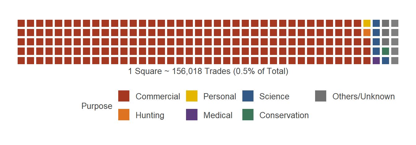
Shockingly, trading due to commercial reasons account for over 94% of all trades! In other words, for every 1 animal traded for conservation purposes, 188 trades are being conducted for profit-making. It seems that conservationists are having difficulties catching up with excess capitalism.
Most Traded Species
The sunburst plot below allows us to find out which animal class, and which species within each class are traded the most:
# Kudos to http://timelyportfolio.github.io/sunburstR/example_baseball.html
# for sunburst reference
trades_by_species <- dataset %>%
                     group_by(Class, Order, Family, Genus, Taxon, CommonName) %>%
                     summarise(total_trades = sum(Qty)) %>%
                     ungroup()

sunburst_input <- trades_by_species %>%
                  group_by(Class) %>%
                  mutate(Node = ifelse(is.na(CommonName),Taxon, gsub("-"," ",CommonName)),
                         Category = Class,
                         CategorySize = sum(total_trades),
                         Seq = paste(Class,Node, sep="-"),
                         Depth = 2) %>%
                  ungroup() %>% group_by(Node, Category, CategorySize, Seq, Depth) %>%
                  summarise(Value = sum(total_trades)) %>%
                  ungroup() %>%
                  # Remove any categories than 0.01 percent since they won't appear anyway
                  filter(CategorySize >= 0.0001 * sum(Value))

# Add Categories That Are Not Represented By A Row
additional_nodes <- sunburst_input %>%
                    mutate(Node = Category,
                           Seq = Category,
                           Depth = 1,
                           Value = 0) %>%
                    unique()

sunburst_input <- rbind(sunburst_input,
                        additional_nodes) %>%
                  arrange(Depth, desc(CategorySize), desc(Value))

# Set the colors for each node
sunburst_palette <- `@c`(palette)(length(unique(sunburst_input$Category)))
names(sunburst_palette) <- unique(sunburst_input$Category)
sunburst_cdomain <- sunburst_input$Node
sunburst_crange <- sapply(1:nrow(sunburst_input),
                          function(i) {
                            node <- sunburst_input[[i,"Node"]]
                            category <- sunburst_input[[i,"Category"]]
                            color <- sunburst_palette[[category]]
                            opacity <- ifelse(category == node, 0.5,0.8)
                            alpha(color,opacity)
                          })

# Plot!
sunburst_plot <- sunburst(sunburst_input %>% select(Seq, Value) ,
                          colors = list(domain=sunburst_cdomain, range=sunburst_crange),
                          count = TRUE,
                          legend = FALSE,
                          width = 600)

# Centerize the sunburst plot
htmlwidgets::onRender(
    sunburst_plot,
    "
    function(el, x) {
    $('.sunburst-chart').css('width', 'initial');
    $('.sunburst-chart').css('height', 'initial');
    $('.sunburst-chart').css('left', '50%');
    $('.sunburst-chart').css('transform', 'translate(-50%, 0)');
    }
    "
)By scrolling through the chart above, we know that Anthozoa accounts for close to 33% of the total trades. Some examples of species belonging to this class are soft and hard corals. The well-publicized African Elephant, belonging to the Mammalia class, interestingly accounts for less than 0.4% of the total trades.
Demand Hotspots
Using export and import data, we can estimate the consumption of wildlife in each country. If a country imports more than it exports, then it is reasonable to assume that the difference is consumed locally.
# Shape Files Courtesy of
# http://thematicmapping.org/downloads/world_borders.php
world_borders <- st_read( dsn= paste0(getwd(),"/",specs_dir,"world_borders") ,
                          layer="TM_WORLD_BORDERS_SIMPL-0.3",
                          quiet = TRUE)
# Revise some of the country names
world_borders <- world_borders %>%
                      left_join(read.csv(paste0(specs_dir, "revised_country_names.csv"),sep = "|"), by="NAME") %>%
                      mutate(NAME = ifelse(is.na(UPDATE_NAME),NAME, UPDATE_NAME)) %>%
                      select(-UPDATE_NAME)

# Dataset containing trades_by_country
trades_by_import <- dataset %>%
                    group_by(Importer) %>%
                    summarise(imports = sum(Qty))
trades_by_export <- dataset %>%
                    group_by(Exporter) %>%
                    summarise(exports = sum(Qty))
trades_by_country <- trades_by_import %>%
                      full_join(trades_by_export, by=c("Importer" = "Exporter")) %>%
                      mutate(imports = ifelse(is.na(imports),0,imports),
                             exports = ifelse(is.na(exports),0,exports),
                             net_imports = ifelse(imports > exports, imports - exports, NA),
                             net_exports = ifelse(exports > imports, exports - imports, NA))

get_leaflet_plot <- function(trade_dataset, isImport = TRUE) {
  # Example Plot Courtesy of
  # https://www.r-graph-gallery.com/183-choropleth-map-with-leaflet/

  map_unt <- ifelse(isImport,"Net Imports","Net Exports")
  map_col <- ifelse(isImport,"red","purple")
  leg_tit <- ifelse(isImport,"Wildlife Demand by Countries (Quantile)","Wildlife Supply by Countries (Quantile)")

  trade_dataset["net_val"] <- ifelse(isImport, trade_dataset["net_imports"], trade_dataset["net_exports"])

  # Join trade information into world data
  polygons <- world_borders %>%
                   left_join(trade_dataset, by=c("ISO2"="Importer")) %>%
                   mutate(rank = rank(desc(net_val),ties="first"))

  # Remove those countries with no wildlife trades
  polygons <- polygons[!is.na(polygons$net_val),]


  # Create leaflet arguments
  # Prevent zooming out infinitely
  leaflet_ptOptions <- providerTileOptions(minZoom = 1)
  # Get colors of each polygon based on trading intensity
  leaflet_palette <- colorQuantile(c(`@c_`(map_col,0.1),`@c_`(map_col)),
                                   polygons$net_val,
                                   n = 5,
                                   na.color = "#ffffffff")
  # What happens to polygon fill when we hover on it
  leaflet_highlightOptions <- highlightOptions(
                                fillOpacity = 0.5,
                                bringToFront = TRUE)
  # Toppltip to appear on hovering
  leaflet_labels <-  sprintf(
                        paste0("<span style='font-family: var(--heading-family); font-size: 1.2em'>%s</span><br/>",
                               "Ranked <span style='font-size:1.2em'>%s</span> (out of %s)<br/>",
                               "%s %s"),
                        polygons$NAME,
                        sapply(polygons$rank, toOrdinal),
                        length(polygons$rank),
                        comma(round(polygons$net_val)),
                        map_unt) %>%
                      lapply(htmltools::HTML)
  # Change background color and foreground color based on fill of the hovered area
  leaflet_labelOptions <- lapply(leaflet_palette(polygons$net_val), function (c){
                            luminosity <- as(hex2RGB(c), "polarLUV")@coords[1]
                            fg_color <- ifelse(luminosity <= 70, `@c`(bg), `@c`(txt))
                            labelOptions(
                              style = list("background-color" = c,
                                           "font-family" = `@f`,
                                           "font-weight" = "normal",
                                           "color" = fg_color,
                                           "border-width" = "thin",
                                           "border-color" = fg_color),
                              textsize = "1em",
                              direction = "auto")
                          })

  # Markers for Top 5 countries
  marker_data <- polygons[polygons$rank <= 5,]
  # Create icons for the Top 5
  marker_icons <- awesomeIcons(
                    # To prevent bootstrap 3.3.7 from loading and removing cosmo theme css, metadata for mobile
                    library = 'fa',
                    markerColor = 'gray',
                    text = sapply(marker_data$rank, function(x) {
                      sprintf("<span style='color: %s; font-size:0.8em'>%s</span>", `@c`(bg), toOrdinal(x)) }),
                    fontFamily = `@f`
                  )
  # Options when marker is clicked
  marker_options <- markerOptions(opacity = 0.9)
  # What to show when marker is clicked
  marker_popup <- sprintf(
                    paste0("<span style='font-family: var(--font-family); color: %s'>[%s] <span style='font-family: var(--heading-family); color: %s; font-size: 1.2em'>%s</span><br/>",
                           "%s %s</span>"),
                    `@c`(txt),
                    sapply(marker_data$rank, toOrdinal),
                    `@c_`(map_col),
                    marker_data$NAME,
                    comma(round(marker_data$net_val)),
                    map_unt) %>%
                    lapply(htmltools::HTML)

  # Create Leaflet plot
  leaflet(polygons, width = "100%") %>%
    addTiles('https://{s}.basemaps.cartocdn.com/light_all/{z}/{x}/{y}.png',options = leaflet_ptOptions) %>%
    setMaxBounds(-200, 100,200,-100) %>%
    setView(0, 30, 1) %>%
    addPolygons(stroke = FALSE,
                fillOpacity = 0.8,
                fillColor = ~leaflet_palette(net_val),
                highlight = leaflet_highlightOptions,
                label = leaflet_labels,
                labelOptions = leaflet_labelOptions) %>%
    addLegend(pal = leaflet_palette,
              values = ~net_val,
              opacity = 0.7,
              title = leg_tit,
              position = "bottomleft") %>%
    addAwesomeMarkers(~LON, ~LAT,
                      data = marker_data,
                      icon = marker_icons,
                      options = marker_options,
                      popup = marker_popup)
}

leaflet_import_plot <- get_leaflet_plot(trades_by_country)

leaflet_import_plot
By utilizing net imports as a proxy, we determined countries with the highest wildlife demand. Surprisingly, China is ranked third, while the United States has around 3 times more demand than the second-ranked country, Japan! Korea and Hong Kong make up the top 5.
It remains to be seen whether the huge gap between United States and the other top 4 countries is due to actual trading or higher diligence in reporting.
Wildlife Supply
Using the opposite logic as demand, if a country exports more than it imports, then we assume that the difference is captured locally.
leaflet_export_plot <- get_leaflet_plot(trades_by_country, FALSE)

leaflet_export_plot
Using net exports as a proxy, we can determine the distribution of supply across the globe. As expected, Southeast Asia, Africa and South America are areas where the majority of wildlife is coming from. In particular, Indonesia exports the most wildlife, close to 2 times than the second-ranked Ecuador. Morocco, the highest-ranked nation in Africa, is 5th.
Identifying the Major Players
For the purposes of this analysis, the major players in the endangered wildlife trade are countries which take part extensively as either suppliers, consumers or intermediaries. In this section, we will aim to:
- surface players that were otherwise overlooked, and
- rank each player according to its wildlife trading activities.
[1] will allow us to have a more macro perspective on each country’s role towards species degradation, while [2] will help us prioritize which countries to focus on given limited conservation resources.
Choosing the Algorithm
The most straightforward way to identify major players is by their net imports/exports. By ordering these metrics, we can potentially find countries supplying and consuming endangered wildlife goods. However, one potential pitfall of such an approach is that the intermediary players get overlooked. Consider the following scenario:
grViz(paste0("
  digraph expInt {

    # Default Specs
    graph [compound = true, nodesep = .5, ranksep = .25]
    node [fontname = '",`@f`,"', fontsize = 14, fontcolor = '",`@c`(bg),"', penwidth=0, color='",`@c`(ltxt),"', style=filled, shape = oval]
    edge [fontname = '",`@f`,"', fontcolor = '",`@c`(ltxt),"', color='",`@c`(ltxt),"']

    Country_A [label = 'Country\nA', fillcolor = '",`@c`(1),"']
    Country_B [label = 'Country\nB', fillcolor = '",`@c`(2),"']
    Country_C [label = 'Country\nC', fillcolor = '",`@c`(3),"']
    { rank = same; Country_A, Country_B, Country_C }

    Country_A -> Country_B [ label='100' ]
    Country_B -> Country_C [ label='99' ]

  }
"), width=309, height=50)
In such a scenario, A will have a net export of 100, B a net import of 1 and C a net import of 99. Using the net import/export approach, B is the least important player. However, in actuality, B should be the most pivotal country as it is involved in all 199 trades. Hence, a better approach is required.
Another way to tackle the issue above is to instead use each country’s gross imports + exports. This approach would work well in the above case, as B would rightly be identified as the most important player. However, one weakness of such a method would be the assumption that absolute numbers are extremely accurate. In truth, this may not be the case, due to the following reasons:
- There may be reporting errors in the CITES database, and
- There could be conversion errors incurred in the Pre-Processing stage.
Moreover, consider the following scenario:
grViz(paste0("
  digraph expInt {

    # Default Specs
    graph [compound = true, nodesep = .5, ranksep = .25]
    node [fontname = '",`@f`,"', fontsize = 14, fontcolor = '",`@c`(bg),"', penwidth=0, color='",`@c`(ltxt),"', style=filled, shape = oval]
    edge [fontname = '",`@f`,"', fontcolor = '",`@c`(ltxt),"', color='",`@c`(ltxt),"']

    Country_A [label = 'Country\nA', fillcolor = '",`@c`(1),"']
    Country_B [label = 'Country\nB', fillcolor = '",`@c`(2),"']
    Country_C [label = 'Country\nC', fillcolor = '",`@c`(3),"']
    Country_D [label = 'Country\nD', fillcolor = '",`@c`(4),"']
    Country_E [label = 'Country\nE', fillcolor = '",`@c`(5),"']

    Country_A -> Country_B [ label='  100' ]
    Country_B -> Country_C [ label='  99' ]
    Country_A -> Country_D [ label='  200' ]
    Country_D -> Country_E [ label='  99' ]
  }
"), width=173, height=200)
Using the imports + exports approach, we conclude that both C and E have the same degree of involvement. However, if the numbers presented are only roughly accurate, it would be reasonable to assume that E is more involved as it is linked to a bigger intermediary in D. (This same argument could be made for drug trafficking, where the closer you are to a drug cartel, the more likely you are to be a major player.)
Fortunately, we can resolve these two issues using Google’s PageRank algorithm. The algorithm is famous for ranking a website’s quality based on:
- the number of links pointing to the website, and
- who is pointing to the website.
This algorithm can be leveraged for our analysis to assess the involvement of a country by:
- the number of trades the country is involved in, and
- which other nations the country is involved with.
Modeling Wildlife Trade
To run the PageRank algorithm, we need to model the wildlife trade as a network, with the countries represented as vertices. Two countries are connected by an edge if the two trade with one another. The degree of wildlife trading between two countries defines the weight of the edge. For the purposes of this study, we will use the sum of imports and exports as the edges’ weights.
Using the above definitions, we are now equipped to model the wildlife trade for the period of 2001 to 2015:
max_label_char <- 20
vertices <- unique(c(dataset$Importer,dataset$Exporter)) %>%
            sort() %>%
            { data.frame(index=.)} %>%
            inner_join(world_borders, by=c("index"="ISO2")) %>%
            # Create labels that truncate names
            mutate(NAME_SHORT = ifelse(nchar(NAME) >= max_label_char, sprintf("%s...",substr(NAME,1,max_label_char - 3)), NAME),
                   REGION = paste0("REGION-",REGION),
                   SUBREGION = paste0("SUBREGION-",SUBREGION)) %>%
            arrange(REGION, SUBREGION)

edges <- dataset %>%
         filter(Importer %in% vertices$index &
                  Exporter %in% vertices$index &
                  Importer != Exporter) %>%
         mutate(v1 = ifelse(Importer < Exporter, Importer, Exporter),
                v2 = ifelse(Importer < Exporter, Exporter, Importer)) %>%
         group_by(v1,v2) %>%
         summarise(total_trades = sum(Qty))

# Calculate imports + exports of each country
vertices$VALUE <- sapply(vertices$index, function(i) { sum(edges[edges$v1 == i | edges$v2 == i,]$total_trades) })

# Filter Top X Countries If Necessary
input_vertices <- vertices
input_edges <- edges %>% filter(v1 %in% input_vertices$index & v2 %in% input_vertices$index)

# Huge thanks to R Graph Gallery for Template
# https://www.r-graph-gallery.com/hierarchical-edge-bundling/

# Create Inputs For The Model
# Color palette for edges and input_vertices
color_dictionary <- `@c`(palette)(length(unique(input_vertices$REGION)))
names(color_dictionary) <- unique(input_vertices$REGION)
n_points <- 100

# Graph Creation
hierarchy <- rbind(input_vertices %>% mutate(parent="root") %>% select(parent,child=REGION) %>% unique(),
                   input_vertices %>% select(parent=REGION,child=SUBREGION) %>% unique(),
                   input_vertices %>% select(parent=SUBREGION, child=index))

# Node Specifications
nodes <- data.frame(name = unique(c(as.character(hierarchy$parent), as.character(hierarchy$child)))) %>%
         left_join(input_vertices %>% select(index, label=NAME_SHORT, region=REGION, value=VALUE), by=c("name"="index")) %>%
         mutate(ranking=rank(value,ties.method="first"))

# Edge Specifications
connections <- data.frame(from=match(input_edges$v1, nodes$name),
                          to=match(input_edges$v2, nodes$name),
                          weights=input_edges$total_trades)

total_trade_min_cutoff <- quantile(input_edges$total_trades, 0.5)
total_trade_max_cutoff <- quantile(input_edges$total_trades, 0.999)
connections$alpha <- lapply(1:nrow(input_edges),
                        function(i) {
                          a <- max(min((input_edges$total_trades[i] - total_trade_min_cutoff) / (total_trade_max_cutoff - total_trade_min_cutoff),1.),0.)
                          list(rep(a,n_points))})

connections$colors <- lapply(1:nrow(input_edges),
                        function(i) {
                          v1 <- input_edges[[i,"v1"]]
                          v2 <- input_edges[[i,"v2"]]

                          # Set up colors
                          region_v1 <- (input_vertices %>% filter(index == v1))$REGION
                          region_v2 <- (input_vertices %>% filter(index == v2))$REGION
                          list(colorRampPalette(c(color_dictionary[[region_v1]],color_dictionary[[region_v2]]))(n_points))

                      })

# Plot the Graph
edge_bundle_graph <-graph_from_data_frame(hierarchy, vertices = nodes)
edge_bundle_plot <- ggraph(edge_bundle_graph, layout="dendrogram", circular=TRUE) +
                    theme_void() +
                    theme_lk(TRUE, TRUE, FALSE, FALSE)

# Add Edge Bundles
# There is a bug in ggraph_1.0.0.9999 where geom_conn_bundle can only plot at most 2 nodes of from before messing up the coloring,
# we will fix this by generating geom_conn_bundle one node at a time
for (v1 in unique(connections$from)) {
  tmp <- connections %>% filter(from == v1)
  edge_bundle_plot <- edge_bundle_plot +
                      geom_conn_bundle(data=get_con(from = tmp$from, to = tmp$to),
                                       colour=unlist(tmp$colors),
                                       alpha=unlist(tmp$alpha),
                                       n = n_points,
                                       tension = 0.8)

}

# Adjust the angle and horizontal alignment of nodes based on the position of x and y
edge_bundle_plot$data["angle"] <- sapply(1:nrow(edge_bundle_plot$data),
                                       function (i) {
                                          t_ratio <- min(max(edge_bundle_plot$data$y[i] / edge_bundle_plot$data$x[i], -10000),10000)
                                          atan(t_ratio) * 180 / pi
                                        })
edge_bundle_plot$data["hjust"] <- sapply(edge_bundle_plot$data$x,
                                         function (x) {
                                           ifelse(x < 0, 1, 0)
                                         })
# Add Node Points
edge_bundle_plot <- edge_bundle_plot +
                    # Create Nodes
                    geom_node_point(aes(filter = leaf, x = x, y=y, colour=region, size=value), alpha=0.8) +
                    geom_node_text(aes(filter = leaf, x = x*1.05, y=y*1.05,
                                       colour=region, label=label, alpha=ranking,
                                       angle=angle, hjust=hjust), size=2.7) +
                    scale_size_continuous(name="Wildlife Trading Activity (Gross Imports + Exports)",
                                          label=function (v) { sprintf("%.0f mil",v/1000000)},
                                          guide=guide_legend(override.aes = list(color=`@c`(txt), alpha=0.8))) +
                    scale_color_manual(values=color_dictionary, guide="none") +
                    scale_alpha_continuous(limits=c(max(nodes$ranking)-100,max(nodes$ranking)-10), na.value=0.1, guide="none") +
                    # Make sure labels are viewable
                    expand_limits(x = c(-1.30, 1.30), y = c(-1.30, 1.30))

edge_bundle_plot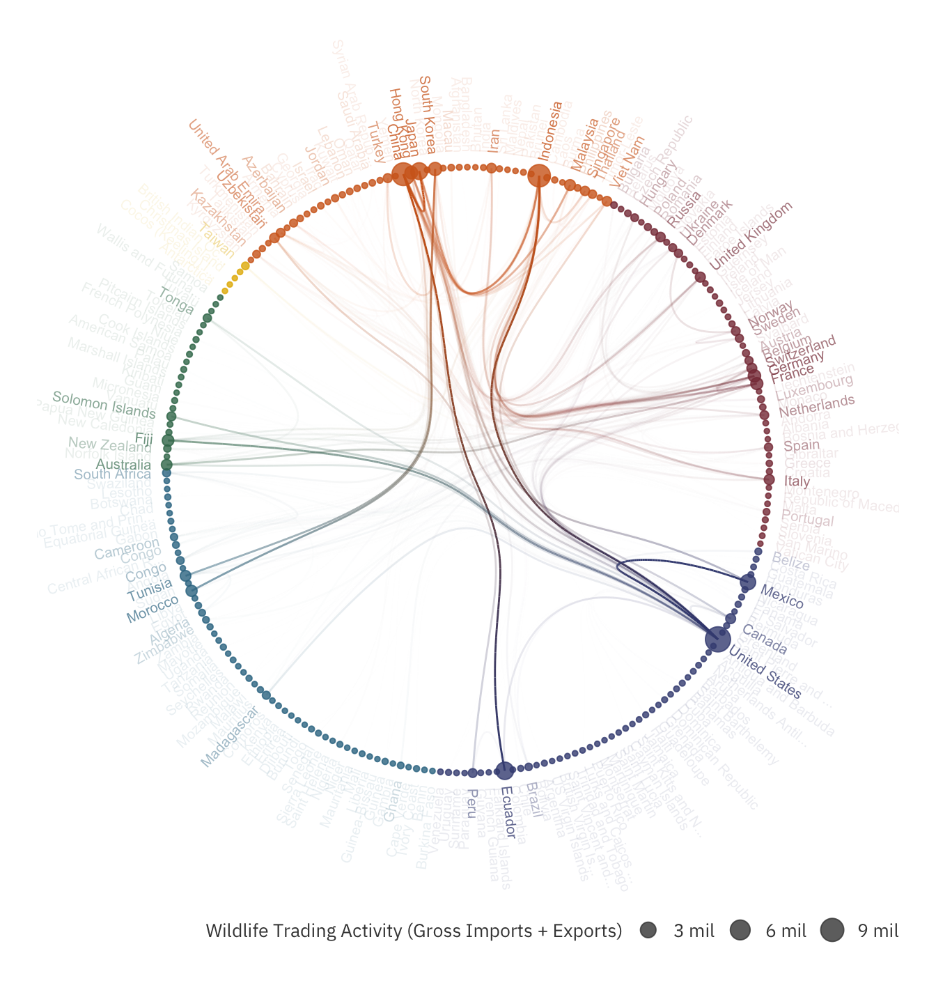
The hierarchical edge bundle plot shows the degree of involvement of each country. The larger the circle, the greater the total imports and exports of the country. Unsurprisingly, United States, China and Indonesia have the highest total imports and exports.
Other than that, we can also identify the most popular trade routes. The larger the wildlife trading, the higher the opacity of that edge. The chart above surfaces some overlooked routes, such as Ecuador to China.
The PageRank Algorithm
With the network constructed, we can proceed to run the PageRank algorithm:
trade_graph <- graph_from_data_frame(edges %>% rename(weight=total_trades), vertices = vertices)
pr_rankings <- page_rank(trade_graph, directed = FALSE)$vector
pr_rankings <- data.frame(index=names(pr_rankings), PRANK=pr_rankings)

# Add rankings to the vertices
vertices <- vertices %>%
            left_join(pr_rankings, by="index") %>%
            mutate(R_PRANK = rank(desc(PRANK),ties.method="first"))

pander(vertices %>% arrange(desc(PRANK)) %>% head(5) %>%
       mutate(Country=NAME, Imports_And_Exports = comma(VALUE), PageRank = percent(PRANK)) %>%
         select(Country, Imports_And_Exports, PageRank),
caption="The Top 5 Major Players According to PageRank")| Country | Imports_And_Exports | PageRank |
|---|---|---|
| United States | 11,161,261 | 16.53% |
| Indonesia | 8,334,342 | 11.72% |
| China | 8,639,113 | 7.57% |
| Japan | 3,765,463 | 3.87% |
| Mexico | 2,845,480 | 3.49% |
Before continuing, it is important for us to understand what the PageRank number represents. When used for assessing the quality of websites, this number refers to a person’s probability of viewing the website. The higher the PageRank probability, the more likely the person will view the website, and hence the higher the quality of the site.
Similarly, in the widlife trading context, the PageRank of a country A is the probability that A is responsible for a wildlife trade. The higher the PageRank of a country, the more wildlife trades are attributed to it. In other words, if there are 1 million trades worldwide, United States would account for approximately 0.165 million trades. By identifying countries with the highest PageRank, we can determine who the major players are.
Comparing With Imports + Exports Approach
To comprehend further, let us first compare PageRank with Imports + Exports:
pr_inputs <- vertices %>%
              mutate(LOG_PRANK = log(PRANK),
                     LOG_VALUE = log(VALUE),
                     # Z value to normalize both
                     Z_PRANK = (LOG_PRANK - mean(LOG_PRANK)) / sd(LOG_PRANK),
                     Z_VAL = (LOG_VALUE - mean(LOG_VALUE)) / sd(LOG_VALUE),
                     # Rankings
                     R_VAL = rank(desc(VALUE), ties.method="first"),
                     R_DIFF = R_PRANK - R_VAL,
                     HAS_DIFF = ifelse(R_DIFF == 0,"NONE",REGION))

hist_input <- select(pr_inputs, Z_VAL, Z_PRANK) %>%
              gather("type","val") %>%
              arrange(desc(type))

hist_plot <- ggplot(hist_input) +
             theme_lk() +
             theme(
               axis.ticks.x = element_blank(),
               axis.title.x = element_blank(),
               axis.text.x = element_blank(),
               axis.line.y = element_blank(),
               axis.ticks.y = element_blank(),
               axis.title.y = element_blank(),
               axis.text.y = element_blank()
             ) +
             scale_x_continuous(expand=c(0,0)) +
             scale_y_continuous(expand=c(0,0)) +
             # Add Mean line
             geom_vline(data=data.frame(1), xintercept = 0, linetype="dashed", colour=`@c`(ltxt)) +
             # Add descriptors
             geom_text(data=data.frame(x=c(0.1,-3,7),
                                        y=c(0.9,0.1,0.1),
                                        hjust=c(0,0,1),
                                        label=c("Mean","Less Important","More Important")),
                        aes(x=x, y=y, hjust=hjust, label=label),
                        colour = `@c`(ltxt),
                        family = `@f`) +
             # Add geom density
             geom_density(aes(x=val, fill=type, colour=type), alpha=0.25) +
             scale_fill_manual(name="Methodology", values=`@c`()[1:2],
                               labels=c("Z_VAL" = "Imports + Exports",
                                        "Z_PRANK" = "PageRank"),
                               guide=guide_legend(override.aes = list(color = `@c`()[1:2]))) +
             scale_color_manual(guide="none", values=`@c`()[1:2])

hist_plot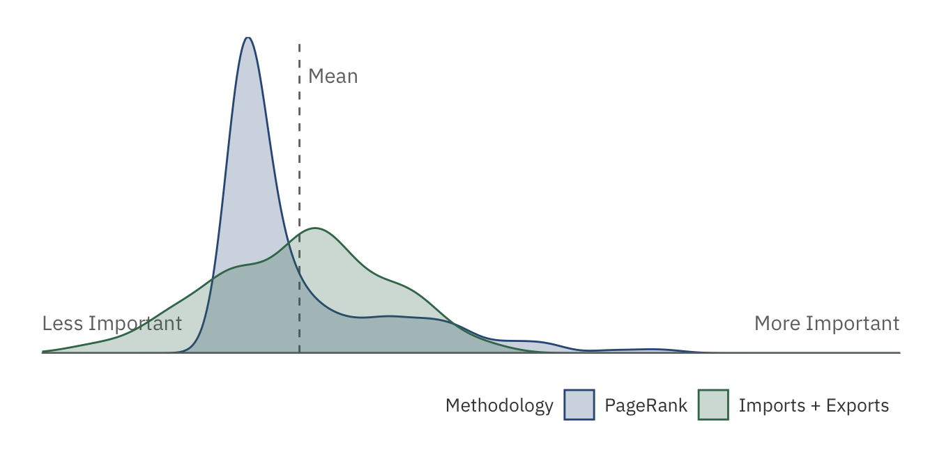
The plot above shows the distribution of PageRank and Imports + Export. The latter distribution has a much gentler slope, implying that wildlife trade responsibilites are more “spread-out” across countries. The PageRank algorithm, however, extremizes this distribution by compacting “average” countries into a single peak. Only a handful of least and most important nations are left in the tails, allowing us to better distinguish them.
Secondly, let us investigate how the rankings shift as we transition from one approach to another:
max_rank <- 25
rank_plot <- ggplot(pr_inputs, aes(colour=HAS_DIFF)) +
              theme_void() +
              theme_lk(TRUE, FALSE, FALSE, FALSE) +
              # Prevent removing points or arrows outside the limit
              coord_cartesian(xlim = c(-2.0,max_rank + 0.5), ylim=c(-1.0,1.7)) +
              # Modify scales
              scale_x_continuous(expand=c(0,0.05)) +
              scale_y_continuous(expand=c(0,0.05)) +
              scale_color_manual(values=c(color_dictionary,"NONE"=`@c`(txt,0.2)),
                                 guide="none") +
              scale_size_continuous(guide="none") +
              # Add descriptors
              geom_text(data=data.frame(x=c(0.2,0.2,1.0,max_rank),
                                        y=c(0,1,-0.9,-0.9),
                                        hjust=c(1,1,0,1),
                                        label=c("Imports\n+ Exports","PageRank",
                                                "More Important","Less Important")),
                        aes(x=x, y=y, hjust=hjust, label=label),
                        colour = `@c`(ltxt),
                        family = `@f`,
                        size = 3) +
              geom_segment(data=data.frame(1),
                           aes(x=max_rank, xend=0.5,y=-0.8,yend=-0.8),
                           colour = `@c`(ltxt),
                           arrow = arrow(length = unit(0.2,"cm"), type="closed")) +
              # Add imports + exports ranks
              geom_text(aes(x=R_VAL, y=-0.1, label=NAME_SHORT), angle=90, hjust=1, size = 3) +
              geom_point(aes(x=R_VAL, y=0, size=Z_VAL), alpha=0.5) +
              # Add pagerank probabilities
              geom_text(aes(x=R_PRANK, y=1.1, label=NAME_SHORT), angle=90, hjust=0, size = 3) +
              geom_point(aes(x=R_PRANK, y=1.0, size=Z_PRANK), alpha=0.5) +
              # Add arrows
              geom_segment(aes(x=R_VAL, xend=R_PRANK, y=0.1, yend=0.9),
                           arrow = arrow(length = unit(0.2, "cm"), type="closed"))

rank_plot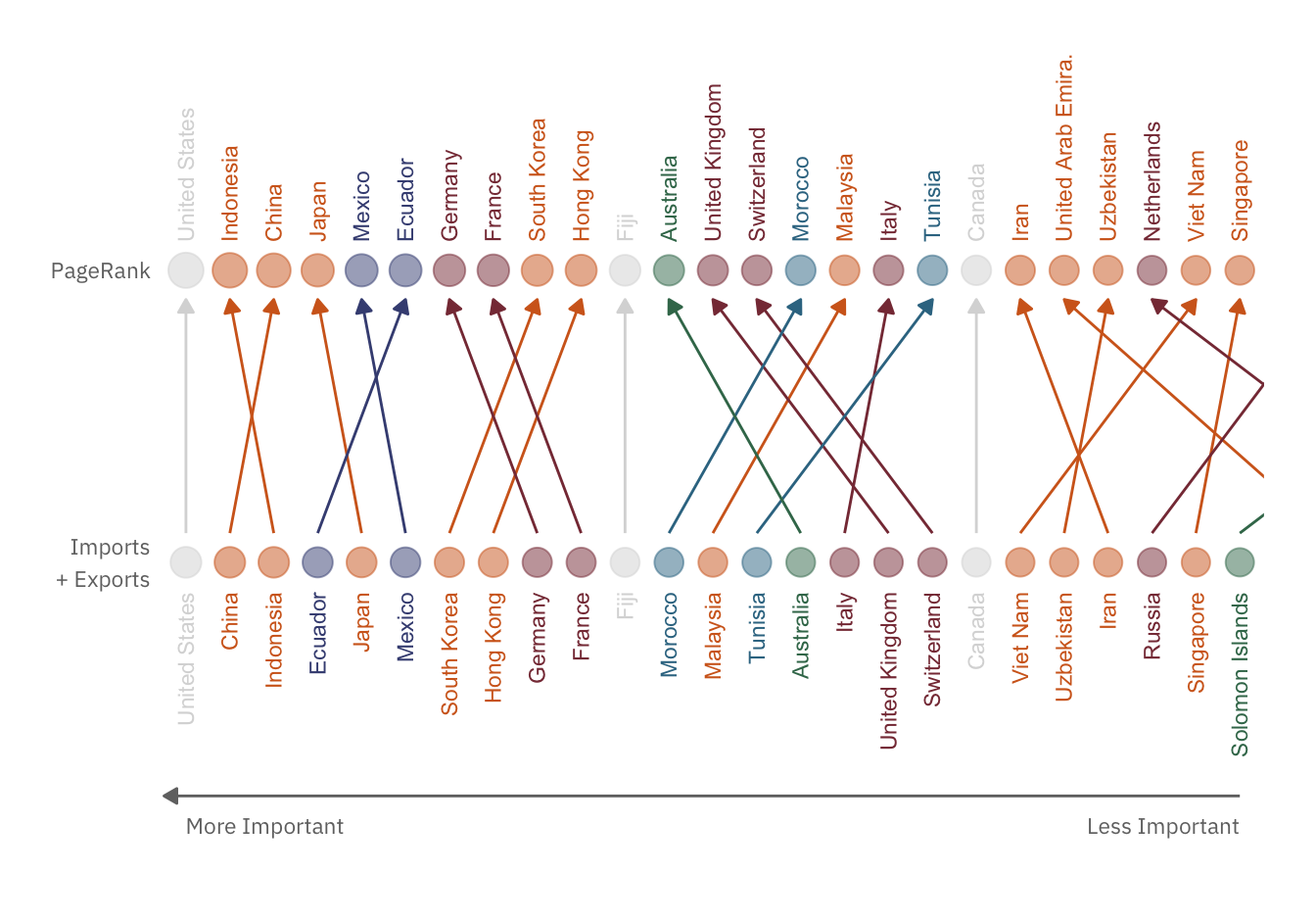
In both rankings, the top 6 countries remain the same. This implies that imports and exports do play a prominent role in the PageRank algorithm. However, the shifts in rankings also indicate that total trades is not the only factor influencing PageRank.
To identify other important factors, let us compare two countries that have been promoted and demoted extensively, Japan and Ecuador:
# Get edges only for neighbors of the two countries of interest
c_int <- sort(c("JP","EC"))
tc_edges <- edges %>%
            filter(v1 %in% c_int | v2 %in% c_int) %>%
            filter(!(v1 == c_int[1] & v2 == c_int[2]))

# Get only neighboring vertices
nodes_int <- unique(c(tc_edges$v1, tc_edges$v2))
V1_vertice <- (vertices %>% filter(index == c_int[1]))
V2_vertice <- (vertices %>% filter(index == c_int[2]))
tc_vertices <- vertices %>% filter(index %in% nodes_int & !(index %in% c_int))

# Construct Input
circ_input <- tc_vertices %>%
              mutate(x = rank(desc(PRANK),ties.method="first"),
                     label = NAME_SHORT,
                     theta = 90 - x / nrow(tc_vertices) * 360)
circ_input$hjust <- sapply(circ_input$theta, function(t) { if (t <= -90){1} else {0}})
circ_input$theta <- sapply(circ_input$theta, function (t) { if (t <= -90) { t + 180} else {t}})

# Colors
neighbors_V1 <- (tc_edges %>% filter(v1 == c_int[1] | v2 == c_int[1]) %>% mutate(v = ifelse(v1 == c_int[1],v2,v1)))$v
neighbors_V2 <- (tc_edges %>% filter(v1 == c_int[2] | v2 == c_int[2]) %>% mutate(v = ifelse(v1 == c_int[2],v2,v1)))$v
circ_input$tag <- sapply(tc_vertices$index, function (ix) {
                    if (ix %in% neighbors_V1 & ix %in% neighbors_V2) { "BOTH" }
                    else if (ix %in% neighbors_V1) { c_int[1] }
                    else if (ix %in% neighbors_V2) { c_int[2] }
                    else { "NONE" }
                  })

compare_colors <- c(`@c`(txt,0.2), color_dictionary[[V1_vertice$REGION]],color_dictionary[[V2_vertice$REGION]])
names(compare_colors) <- c("BOTH", c_int)
compare_labels <- c("Both",V1_vertice$NAME,V2_vertice$NAME)
names(compare_labels) <- c("BOTH",c_int)
compare_plot <- ggplot(circ_input, aes(x=x, y=1, size=PRANK, color=tag)) +
                theme_void() +
                theme_lk(TRUE, TRUE, FALSE, FALSE) +
                theme(plot.margin = unit(c(20,0,20,0),'pt')) +
                expand_limits(y = c(0, 1.30)) +
                # Add points, lines and labels of neighboring countries
                geom_point(alpha=0.5) +
                geom_segment(data= circ_input %>% filter(tag %in% c_int),
                             aes(xend=x, y=0, yend=1, alpha=VALUE),
                             size=0.5) +
                geom_text(data= circ_input %>% filter(tag %in% c_int),
                          aes(label=label, angle=theta, hjust=hjust),
                          y = 1.05,
                          size=3,
                          show.legend = FALSE) +
                # Change Legends
                scale_size_continuous(name = "PageRank",
                                      labels = percent) +
                scale_color_manual(name="Traded With",
                                   values = compare_colors,
                                   labels = compare_labels) +
                scale_alpha_continuous(guide="none") +
                # Change to coordinate polar
                coord_polar()

compare_plot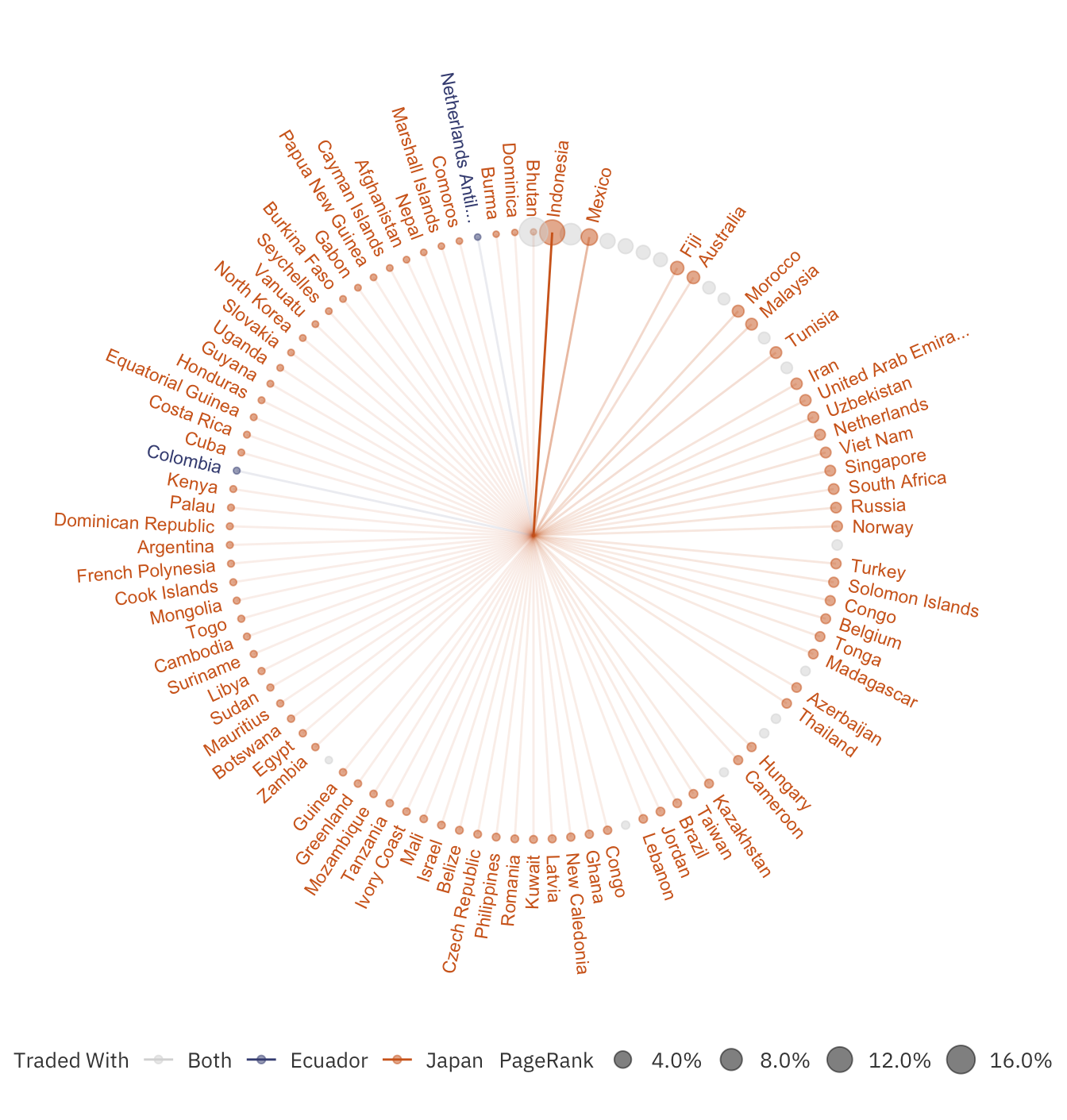
The diagram above shows all the countries that either Japan or Ecuador traded with. It is clear that Japan has a greater outreach than Ecuador, even though the latter has a higher total imports + exports. This degree of outreach caused the algorithm to promote Japan at the expense of Ecuador.
Decomposing PageRank
The PageRank algorithm allows us to determine who the major players are. However, each country has different roles to play. Some can be consumers (countries which fuel the demand of wildlife consumption), suppliers (countries which capture the wildlife and ship them out) or even dealers (intermediaries which connect suppliers and consumers). To reduce wildlife trading effectively, tackling different roles will require different strategies.
In this section, we will construct a method to identify the top consumers, dealers and suppliers. It is important to note that these roles are not exclusive; a country may well be a supplier of one species and a consumer of another.
To determine a country’s role, we will first split the quantity traded of each species into three constituents:
- Net Imports: The amount of trades being brought into the country. This is the leftover amount when we subtract imports with exports. If exports are more than imports, then there are no net imports.
- Net Exports: The amount of trades being shipped out of the country. This is equivalent to the amount remaining when we subtract exports with imports. If imports are more than exports, there are no net exports.
- Transits: These are the trades being brought in and then shipped out of the country. This is equivalent to the minimum of Exports and Imports.
These constitutients are then summed up across species to determine a country’s net imports, net exports and transits. Thee 3 values are subsequently used to decompose PageRank via the following approach:
grViz(paste0("
  digraph decomPR {

    # Default Specs
    graph [compound = true, nodesep = .5, ranksep = .25]
    node [fontname = '",`@f`,"', fontsize = 14, fontcolor = '",`@c`(bg),"', penwidth=0, color='",`@c`(ltxt),"', style=filled, shape = oval]
    edge [fontname = '",`@f`,"', fontcolor = '",`@c`(ltxt),"', color='",`@c`(ltxt),"']

    PageRank [fillcolor = '",`@c`(ltxt),"', shape=diamond]
    ConsumerRank [fillcolor = '",`@c`(red),"']
    DealerRank [fillcolor = '",`@c`(sec),"']
    SupplierRank [fillcolor = '",`@c`(purple),"']

    PageRank -> ConsumerRank [ label=' x Net Imports %' ]
    PageRank-> DealerRank [ label='  x Transit %' ]
    PageRank -> SupplierRank [ label='  x Net Exports %' ]
  }
"), width=405, height=100)
where
- ConsumerRank is the % of trades due to the country’s consumption,
- DealerRank is the % of trades due to the country being an intermediary, and
- SupplierRank is the % of trades due to the country’s provision.
By ordering each of these three ranks, we can determine which countries are the top consumers, dealers and suppliers. Summing up each of these metrics would also allow us to determine the major drivers behind wildlife trading:
# Calculate the Net Exports and Imports for each country at a specified level of taxonomy granularity
net_gross_p_country <- function(granularity="Taxon") {

  imports <- dataset %>%
    group_by_at(vars("Importer", granularity)) %>%
    summarise(Imports = sum(Qty)) %>% ungroup()
  exports <- dataset %>%
    group_by_at(vars("Exporter", granularity)) %>%
    summarise(Exports = sum(Qty)) %>% ungroup()

  by_joins <- c("Exporter",granularity)
  names(by_joins) <- c("Importer",granularity)

  trades <- imports %>%
    full_join(exports, by=by_joins) %>%
    mutate(
      index = Importer,
      Imports = ifelse(is.na(Imports),0,Imports),
      Exports = ifelse(is.na(Exports),0,Exports),
      Gross = Imports + Exports,
      Net_Exports = ifelse(Exports > Imports, Exports - Imports,0),
      Net_Imports = ifelse(Imports > Exports, Imports - Exports,0),
      # Trades that are not supplied [net export] or consumed [net imports] are ones
      # that are being transited within the country
      Transits = ifelse(Imports > Exports, Exports, Imports)
    )
  trades %>% select_at(vars("index",granularity,"Imports","Exports","Gross","Net_Exports","Net_Imports","Transits"))
}
country_taxon_trades <- net_gross_p_country()

# Calculate the demand, supply and dealer rankings for each country using the following:
# ConsumerRank: net imports / gross * PageRank
# SupplierRank: net exports / gross * PageRank
# DealerRank: transits / gross * PageRank
country_add_info <- country_taxon_trades %>%
                      group_by(index) %>%
                      summarise(GROSS = sum(Gross),
                                NET_IMPORTS = sum(Net_Imports),
                                NET_EXPORTS = sum(Net_Exports),
                                TRANSITS = sum(Transits))

vertices <- vertices %>%
            left_join(country_add_info, country_add_info, by="index") %>%
            mutate(
              CRANK = NET_IMPORTS / GROSS * PRANK,
              R_CRANK = rank(desc(CRANK), ties.method="first"),
              DRANK = TRANSITS / GROSS * PRANK,
              R_DRANK = rank(desc(DRANK), ties.method="first"),
              SRANK = NET_EXPORTS / GROSS * PRANK,
              R_SRANK = rank(desc(SRANK), ties.method="first")
            )

"% Trade Contribution by Roles:\n" %>%
paste0(paste0(sapply(c("CRANK","DRANK","SRANK"), function(r) {
    sprintf("%ss: %.2f%%", ifelse(r == "CRANK","Consumer", ifelse(r == "DRANK","Dealer","Supplier")),sum(vertices[r]) * 100)
  }), collapse="\n")) %>%
cat()
## % Trade Contribution by Roles:
## Consumers: 45.81%
## Dealers: 4.07%
## Suppliers: 46.04%From the above summary, consumption and supply of wildlife goods contribute the most to wildlife exchanges. Intermediaries surprisingly do not play major roles. This suggests that to reduce trading, we are better off focusing on reducing supply and demand (instead of breaking down the channels connecting them).
# Normalize each of the ranks so that totals of each rank = 1
leaf_inputs <- vertices %>%
                mutate(
                  CRANK = CRANK / sum(CRANK),
                  DRANK = DRANK / sum(DRANK),
                  SRANK = SRANK / sum(SRANK)
                )

# Get only the top countries to show degree of roles
n_show <- 12
leaf_inputs <- leaf_inputs %>% arrange(desc(PRANK)) %>% head(n_show)
leaf_inputs$NAME <- factor(leaf_inputs$NAME, levels=unique(leaf_inputs$NAME))

# Normalize between the three ranks to make sure that plot is properly "zoomed"
# as free_y is not available for polar coordinates
leaf_inputs$MAXR <- sapply(1:nrow(leaf_inputs), function(i) {
  max(leaf_inputs[i,"CRANK"],leaf_inputs[i,"DRANK"],leaf_inputs[i,"SRANK"])
})
leaf_inputs <- leaf_inputs %>%
                mutate(
                  CRANK = CRANK / MAXR,
                  DRANK = DRANK / MAXR,
                  SRANK = SRANK / MAXR,
                  CLOSE = CRANK
                ) %>%
                gather("Key","Value", CRANK, DRANK, SRANK, CLOSE) %>%
                mutate(
                  Key = ifelse(Key == "CRANK",0,
                               ifelse(Key == "DRANK",120,
                                      ifelse(Key == "SRANK",240,
                                             ifelse(Key == "CLOSE",360,0))))
                ) %>%
                select(NAME, REGION, PRANK, Key, Value)

# Plot!
leaf_plot <- ggplot(leaf_inputs, aes(x=Key, y=Value, fill=REGION, color=REGION)) +
              coord_polar(start=60/180*pi) +
              theme_lk(TRUE, TRUE, FALSE, FALSE) +
              theme(
                axis.line.x = element_blank(),
                axis.ticks.x = element_blank(),
                axis.title.x = element_blank(),
                axis.text.x = element_text(colour=`@c`(ltxt), size = 8, angle=c(-60,0,60)),
                panel.grid.major.x = element_line(colour=`@c`(txt,0.2)),
                axis.line.y = element_blank(),
                axis.ticks.y = element_blank(),
                axis.title.y = element_blank(),
                axis.text.y = element_blank(),
                panel.grid.major.y = element_blank(),
                strip.background = element_blank(),
                strip.text.x = element_blank()
              ) +
              scale_x_continuous(limits=c(0,360),
                                 breaks = c(0,120,240),
                                 labels=c("Consumer","Dealer","Supplier"),
                                 minor_breaks = NULL) +
              scale_y_continuous(limits=c(0,NA)) +
              scale_fill_manual(values = color_dictionary, guide = "none") +
              scale_color_manual(values = color_dictionary,guide = "none") +
              geom_area(alpha=0.2, size=0) +
              geom_text(data=leaf_inputs %>% select(NAME, REGION) %>% unique(),
                        aes(label=NAME),
                        x=0,y=0,
                        family=`@f`,
                        alpha=0.9) +
              facet_wrap(~NAME)

suppressWarnings(leaf_plot)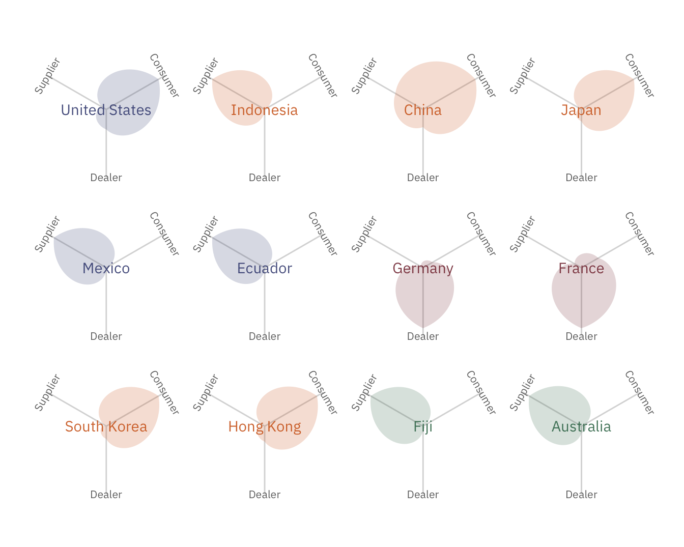
The leaf plots above show the roles played by the top 12 countries. United States, the biggest player, are mostly consumers, while Germany is a large dealer. China unsurprisingly is both consuming and supplying wildlife resources.
The Major Players
Listed below are the top consumers, dealers and suppliers detected through the PageRank algorithm.
to_text <- function (data) {
  tmp <- data %>% head(5)
  tmp$NAME
}

consumers <- vertices %>% arrange(R_CRANK)
dealers <- vertices %>% arrange(R_DRANK)
suppliers <- vertices %>% arrange(R_SRANK)

players <- data.frame("Consumers"=to_text(consumers),
                      "Dealers"=to_text(dealers),
                      "Suppliers"=to_text(suppliers))

pander(players, caption="The Top Suppliers, Dealers and Consumers")| Consumers | Dealers | Suppliers |
|---|---|---|
| United States | Germany | Indonesia |
| China | United States | Mexico |
| Japan | Switzerland | Ecuador |
| South Korea | France | China |
| Hong Kong | United Arab Emirates | Fiji |
To find out more about each country’s trading activities, please hover or click on the buttons below:


Summary of Results
By standardizing terms through the roll-up median approach and ranking countries via the PageRank algorithm, we have identified the major players in endangered wildlife trade:
- Consumers are countries which generate the demand for wildlife. It is important to educate citizens in these countries to stop using wildlife products. The top 5 consumers are United States, China, Japan, South Korea, Hong Kong.
- Dealers are countries which connect suppliers to consumers. More stringent measures can be set up in the trading ports to reduce endangered wildlife trading. The top 5 dealers are Germany, United States, Switzerland, France, United Arab Emirates.
- Suppliers are countries that provide wildlife goods. Efforts to protect the nature reserves of these countries should be emphasized. The top 5 suppliers are Indonesia, Mexico, Ecuador, China, Fiji.
Limitations
The above analysis, though simplified, provides us with a better picture of the wildlife situation across the world. Listed below are some suggestions to improve the accuracy of results:
- One Side of the Story: This study is based on data reported by governments. As such, many black market trades are missing. It would be interesting to identify these “shadow” trades by verifying the consistency of the CITES data, before integrating them back into this analysis.
- Wild: Due to size constraints, we only considered trades whose sources are tagged as “Wild”. By expanding the scope, additional insights could be unearthed.
- Species-Specific Fixes: The methods in pre-processing are generalized and favor expediency over accuracy. By fixing each trade according to individual species’s characteristics (such as weight), we can obtain more accurate transformations of the terms into animal counts.
References
CITES Database 2017. https://www.cites.org. Downloaded on 24 April 2018.
IUCN 2017. The IUCN Red List of Threatened Species. Version 2017-3. http://www.iucnredlist.org. Downloaded on 25 April 2018.